Time-frequency representations

Most source separation algorithms do not their operations in the time domain, but rather in the frequency domain. For this, nussl provides an interface for working with Short-Time Fourier Transform (STFT) data. Here, we describe how to do some simple STFT operations with the :class:nussl.AudioSignal object. Other time-frequency representations such as the constant-Q transform are not in nussl at this time.

STFT Basics

Let’s reinitialize signal1 from the previous page. We should be able to get frequency domain data by looking at signal1.stft_data. Let’s try that.

import nussl
import time
start_time = time.time()

input_file_path = nussl.efz_utils.download_audio_file(
    'schoolboy_fascination_excerpt.wav')
signal1 = nussl.AudioSignal(input_file_path)
print('STFT Data:', signal1.stft_data)

Matching file found at /home/pseetharaman/.nussl/audio/schoolboy_fascination_excerpt.wav, skipping download.
STFT Data: None

Whoops! Because this object was initialized from a .wav file (i.e., time-series data), this :class:AudioSignal: object has no frequency domain data by default. To populate it with frequency data we do thusly:

stft = signal1.stft()
print(stft.shape)

(1025, 1293, 2)

Aha! Now we can examine how STFT data is stored in the :class:AudioSignal: object. Similar to signal1.audio_data, STFT data is stored in a (complex-valued) numpy array called signal1.stft_data.

By inspecting the shape we see that the first dimension represents the number of FFT bins taken at each hop, the second represents the length of our signal (in hops), and the third dimension is number of channels.

We can also get power spectrogram data from our signal as well. As we would expect, this is the same shape as signal1.stft_data.

# np.abs(signal1.stft_data) ** 2
psd = signal1.power_spectrogram_data
print(psd.shape)

(1025, 1293, 2)

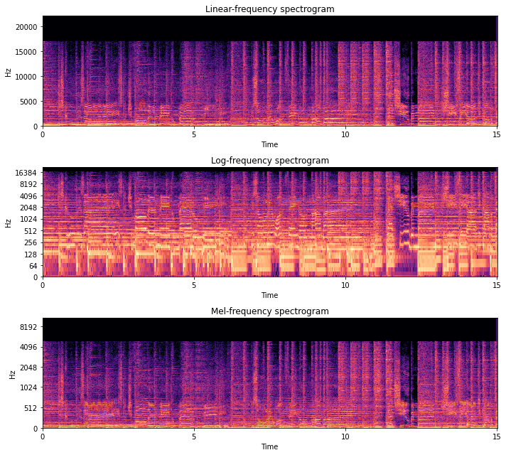
Let’s take a look at the spectrogram, using some helpful functions from nussl.utils, with different settings on the y_axis.

import matplotlib.pyplot as plt

plt.figure(figsize=(10, 9))
plt.subplot(311)
plt.title('Linear-frequency spectrogram')
nussl.utils.visualize_spectrogram(signal1)

plt.subplot(312)
plt.title('Log-frequency spectrogram')
nussl.utils.visualize_spectrogram(signal1, y_axis='log')

plt.subplot(313)
plt.title('Mel-frequency spectrogram')
nussl.utils.visualize_spectrogram(signal1, y_axis='mel')

plt.tight_layout()
plt.show()

Inverse STFTs

Let’s do something a little more interesting with our :class:AudioSignal: object. Since signal1.stft_data is just a regular numpy array, we can access and manipulate it as such. So let’s implement a low pass filter by creating a new :class:AudioSignal: object and leaving signal1 unaltered.

Let’s eliminate all frequencies above about 400 Hz in our signal.

import numpy as np

lp_stft = signal1.stft_data.copy()
lp_cutoff = 1000  # Hz
frequency_vector = signal1.freq_vector  # a vector of frequency values for each FFT bin
idx = (np.abs(frequency_vector - lp_cutoff)).argmin()  # trick to find the index of the closest value to lp_cutoff
lp_stft[idx:, :, :] = 0.0j  # every freq above lp_cutoff is 0 now

Okay, so now we have low passed STFT data in the numpy array lp_stft. Now we are going to see how we can initialize a new :class:AudioSignal: object using this data. Let’s make a copy of the original signal, signal1, using its helper function make_copy_with_stft_data:

signal1_lp = signal1.make_copy_with_stft_data(lp_stft)
print('Audio Data:', signal1_lp.audio_data)

Audio Data: None

Easy-peasy! Now signal1_lp is a new :class:AudioSignal: object that has been initialized with STFT data instead of time series data. But there’s no audio data to listen to! Before we can hear the result, we need to do an Inverse STFT to get back time-series data:

signal1_lp.istft()
signal1_lp.embed_audio()
print(signal1_lp)

AudioSignal (unlabeled): 15.000 sec @ /home/pseetharaman/.nussl/audio/schoolboy_fascination_excerpt.wav, 44100 Hz, 2 ch.

Let’s check out what the spectrogram looks like.

import matplotlib.pyplot as plt

plt.figure(figsize=(10, 3))
plt.title('Masked spectrogram')
nussl.utils.visualize_spectrogram(signal1_lp, y_axis='mel')
plt.show()

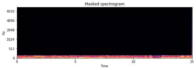
Cool beans!

STFT Parameters

Where did the STFT parameters for our audio signals come from? There are three main arguments for taking an STFT:

1. window_length: How long are the windows within which to take the FFT?

2. hop_length: How much to hop between windows?

3. window_type: What sort of windowing function to use?

These three parameters are grouped into a namedtuple object that belongs to every AudioSignal object. This is the STFTParams object:

nussl.STFTParams

nussl.core.audio_signal.STFTParams

When we created the audio signals above, the STFT parameters were built on initialization:

signal1.stft_params

STFTParams(window_length=2048, hop_length=512, window_type='sqrt_hann')

The STFT parameters are built using helpful defaults based on properties of the audo signal. 32 millisecond windows are used with an 8 millisecond hop between windows. At 44100 Hz, this results in 2048 for the window length and 512 for the hop length. The window type is the sqrt_hann window, which generally has better separation performance. There are many windows that can be used:

nussl.constants.ALL_WINDOWS

['hamming', 'rectangular', 'hann', 'blackman', 'triang', 'sqrt_hann']

An AudioSignal’s STFT parameters can be set after the fact. Let’s change the one for signal1:

signal1.stft_params = nussl.STFTParams(
    window_length=256, hop_length=128)
signal1.stft().shape

(129, 5169, 2)

The shape of the resultant STFT is now different. Note that 256 resulted in 129 frequencies of analysis per frame. In general, the rule is (window_length // 2) + 1.

end_time = time.time()
time_taken = end_time - start_time
print(f'Time taken: {time_taken:.4f} seconds')

Time taken: 7.7818 seconds