Separation via Time-Frequency Masking

One of the most effective ways to separate sounds from a mixture is by masking. Consider the following mixture, which we will download via one of the dataset hooks in nussl.

import nussl
import matplotlib.pyplot as plt
import numpy as np
import copy

import time
start_time = time.time()

musdb = nussl.datasets.MUSDB18(download=True)

item = musdb[40]
mix = item['mix']
sources = item['sources']

Let’s listen to the mixture. Note that it contains 4 sources: drums, bass, vocals, and all other sounds (considered as one source: other).

mix.embed_audio()
print(mix)

AudioSignal (unlabeled): 6.803 sec @ James May - Dont Let Go, 44100 Hz, 2 ch.

Let’s now consider the time-frequency representation of this mixture:

plt.figure(figsize=(10, 3))
plt.title('Mixture spectrogram')
nussl.utils.visualize_spectrogram(mix, y_axis='mel')
plt.tight_layout()
plt.show()

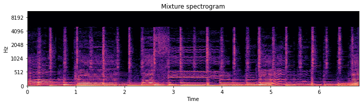
Masking means to assign each of these time-frequency bins to one of the four sources in part or in whole. The first method involves creating a soft mask on the time-frequency representation, while the second is a binary mask. How do we assign each time-frequency bin to each source? This is a very hard problem, in general. For now, let’s consider that we know the actual assignment of each time-frequency bin. If we know that, how do we separate the sounds?

First let’s look at one of the sources, say the drums:

plt.figure(figsize=(10, 3))
plt.title('Drums')
nussl.utils.visualize_spectrogram(sources['drums'], y_axis='mel')
plt.tight_layout()
plt.show()

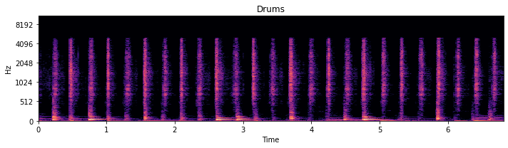
Looking at this versus the mixture spectrogram, one can see which time-frequency bins belong to the drum. Now, let’s build a mask on the mixture spectrogram using a soft mask. We construct the soft mask using the drum STFT data and the mixture STFT data, like so:

mask_data = np.abs(sources['drums'].stft()) / np.abs(mix.stft())

Hmm, this may not be a safe way to do this. What if there’s a 0 in both the source and the mix? Then we would get 0/0, which would result in NaN in the mask. Or what if the source STFT is louder than the mix at some time-frequency bin due to cancellation between sources when mixed? Let’s do things a bit more safely by using the maximum and some checking…

mask_data = (
    np.abs(sources['drums'].stft()) /
    np.maximum(
        np.abs(mix.stft()),
        np.abs(sources['drums'].stft())
    ) + nussl.constants.EPSILON
)

Great, some peace of mind. Now let’s apply the soft mask to the mixture to separate the drums. We can do this by element-wise multiplying the STFT and adding the mixture phase.

magnitude, phase = np.abs(mix.stft_data), np.angle(mix.stft_data)
masked_abs = magnitude * mask_data
masked_stft = masked_abs * np.exp(1j * phase)

drum_est = mix.make_copy_with_stft_data(masked_stft)
drum_est.istft()
drum_est.embed_audio()

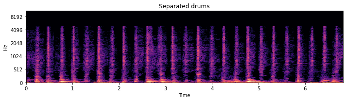
plt.figure(figsize=(10, 3))
plt.title('Separated drums')
nussl.utils.visualize_spectrogram(drum_est, y_axis='mel')
plt.tight_layout()
plt.show()

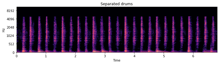
Cool! Sounds pretty good! But it’d be a drag if we had to type all of that every time we wanted to separate something. Lucky for you, we built this stuff into the core functionality of nussl!

SoftMask and BinaryMask

At the core of nussl’s separation functionality are the classes SoftMask and BinaryMask. These are classes that contain some logic for masking and can be used with AudioSignal objects. We have a soft mask already, so let’s build a SoftMask object.

soft_mask = nussl.core.masks.SoftMask(mask_data)

soft_mask contains our mask here:

soft_mask.mask.shape

(1025, 587, 2)

We can apply the soft mask to our mix and return the separated drums easily, using the apply_mask method:

drum_est = mix.apply_mask(soft_mask)
drum_est.istft()
drum_est.embed_audio()

plt.figure(figsize=(10, 3))
plt.title('Separated drums')
nussl.utils.visualize_spectrogram(drum_est, y_axis='mel')
plt.tight_layout()
plt.show()

Sometimes masks are binary instead of soft. To apply a binary mask, we can do this:

binary_mask = nussl.core.masks.BinaryMask(mask_data > .5)
drum_est = mix.apply_mask(binary_mask)
drum_est.istft()
drum_est.embed_audio()

plt.figure(figsize=(10, 3))
plt.title('Separated drums')
nussl.utils.visualize_spectrogram(drum_est, y_axis='mel')
plt.tight_layout()
plt.show()

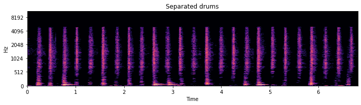
Playing around with the threshold will result in more or less leakage of other sources:

binary_mask = nussl.core.masks.BinaryMask(mask_data > .05)
drum_est = mix.apply_mask(binary_mask)
drum_est.istft()
drum_est.embed_audio()

plt.figure(figsize=(10, 3))
plt.title('Separated drums')
nussl.utils.visualize_spectrogram(drum_est, y_axis='mel')
plt.tight_layout()
plt.show()

You can hear the vocals slightly in the background as well as the other sources.

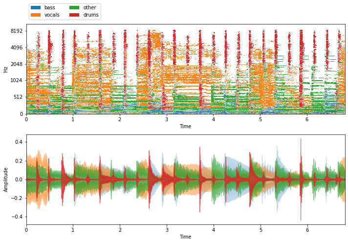
Finally, given a list of separated sources, we can use some handy nussl functionality to easily visualize the masks and listen to the original sources that make up the mixture.

plt.figure(figsize=(10, 7))
plt.subplot(211)
nussl.utils.visualize_sources_as_masks(
    sources, db_cutoff=-60, y_axis='mel')
plt.subplot(212)
nussl.utils.visualize_sources_as_waveform(
    sources, show_legend=False)
plt.tight_layout()
plt.show()

nussl.play_utils.multitrack(sources, ext='.wav')

end_time = time.time()
time_taken = end_time - start_time
print(f'Time taken: {time_taken:.4f} seconds')

Time taken: 27.0189 seconds