Evaluating separation performance
In this notebook, we will demonstrate how one can use nussl to quickly and easily compare different separation approaches. Here, we will evaluate the performance of several simple vocal separation algorithms on a subset of the MUSDB18 dataset.
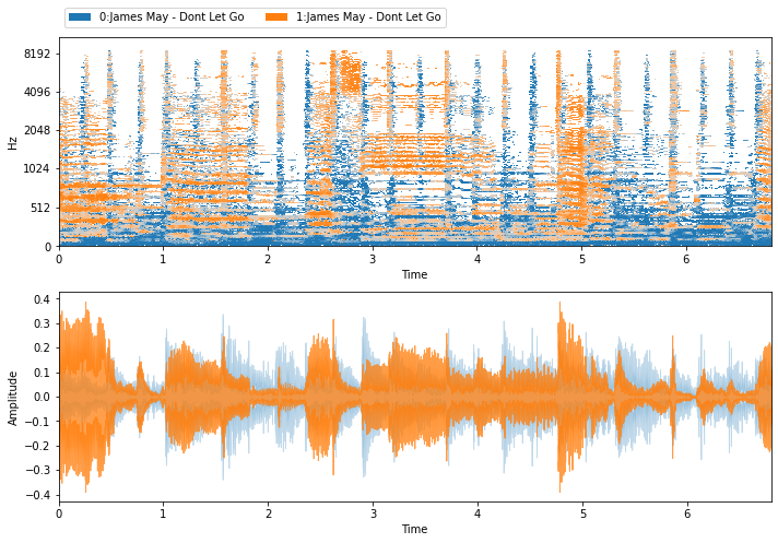
First, let’s load the dataset using nussl’s dataset utilities, and inspect an item from the dataset using nussl’s plotting and playing utlities:
[1]:
import nussl
import numpy as np
import matplotlib.pyplot as plt
import json
import time
start_time = time.time()
# seed this notebook
nussl.utils.seed(0)
# this will download the 7 second clips from MUSDB
musdb = nussl.datasets.MUSDB18(download=True)
i = 40 #or get a random track like this: np.random.randint(len(musdb))
# helper for plotting and playing
def visualize_and_embed(sources):
plt.figure(figsize=(10, 7))
plt.subplot(211)
nussl.utils.visualize_sources_as_masks(
sources, db_cutoff=-60, y_axis='mel')
plt.subplot(212)
nussl.utils.visualize_sources_as_waveform(
sources, show_legend=False)
plt.tight_layout()
plt.show()
nussl.play_utils.multitrack(sources, ext='.wav')
item = musdb[i]
mix = item['mix']
sources = item['sources']
visualize_and_embed(sources)
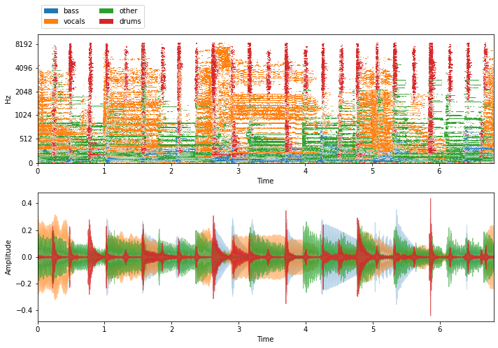
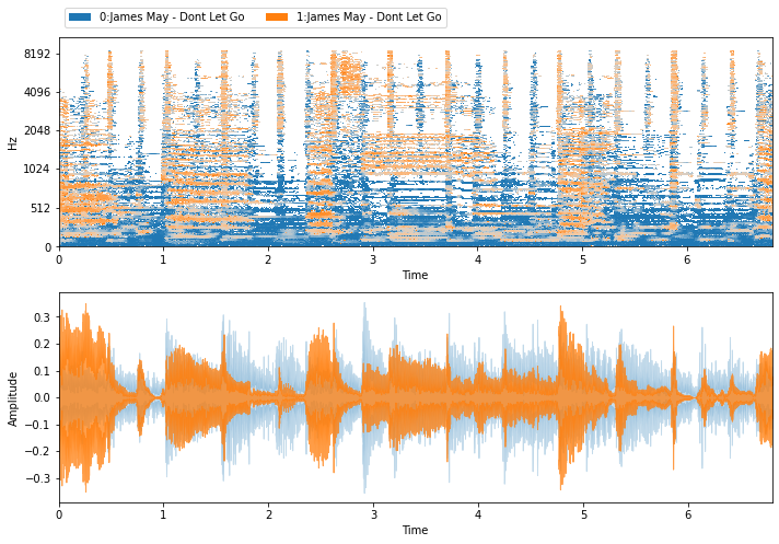
So, there are four sources in each item of the MUSDB18 dataset: drums, bass, other, and vocals. Since we’re doing vocal separation, what we really care about is two sources: vocals and accompaniment (drums + bass + other). So it’d be great if each item in the dataset looked more like this:
[2]:
vocals = sources['vocals']
accompaniment = sources['drums'] + sources['bass'] + sources['other']
new_sources = {'vocals': vocals, 'accompaniment': accompaniment}
visualize_and_embed(new_sources)
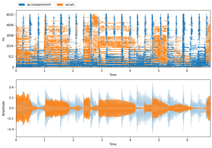
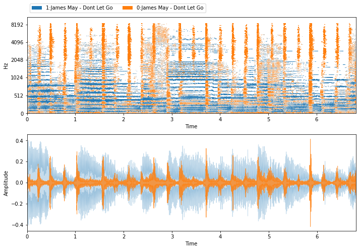
When evaluating vocals separation, what we’ll do is compare our estimate for the vocals and the accompanient to the above ground truth isolated sources. But first, there’s a way in nussl to automatically group sources in a dataset by type, using nussl.datasets.transforms.SumSources:
[3]:
tfm = nussl.datasets.transforms.SumSources([['drums', 'bass', 'other']])
# SumSources takes a list of lists, which each item in the list being
# a group of sources that will be summed into a single source
musdb = nussl.datasets.MUSDB18(download=True, transform=tfm)
item = musdb[i]
mix = item['mix']
sources = item['sources']
visualize_and_embed(sources)
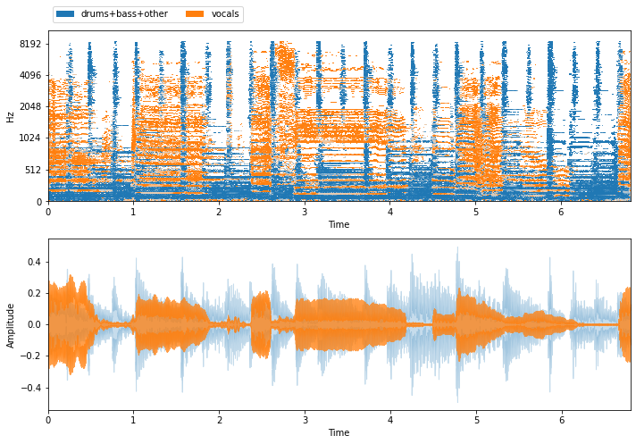
Now that we have a mixture and corresponding ground truth sources, let’s pump the mix through some of nussl’s separation algorithms and see what they sound like!
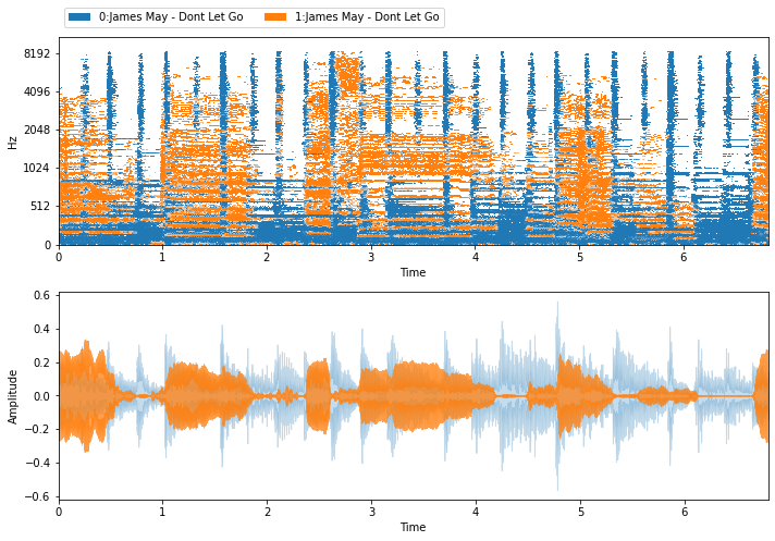
REPET
[4]:
repet = nussl.separation.primitive.Repet(mix)
repet_estimates = repet()
visualize_and_embed(repet_estimates)
2DFT
[5]:
ft2d = nussl.separation.primitive.FT2D(mix)
ft2d_estimates = ft2d()
visualize_and_embed(ft2d_estimates)
HPSS
[6]:
hpss = nussl.separation.primitive.HPSS(mix)
hpss_estimates = hpss()[::-1]
# hpss gives harmonic then percussive
# so let's reverse the order of the list
visualize_and_embed(hpss_estimates)
Putting it all together
Now that we have some estimates, let’s evaluate the performance. There are many ways to do this in nussl:
Original BSS Evaluation metrics:
Source-to-distortion ratio (SDR): how well does the estimate match the ground truth source?
Source-to-interference ratio (SIR): how well does the estimate suppress the other sources?
Source-to-artifact ratio (SAR): how much musical/random noise is in the estimate?
Source to Spatial Distortion Image (ISR): how well does the algorithm keep the source in the same spatial location?
New BSS Evaluation metrics: these metrics are refined versions of the originals and are argued to be more robust.
Precision and recall on binary masks: an older way to evaluate methods is to look at the values of the actual mask and the estimated mask and compute precision/recall over each time-frequency bin.
Let’s extract each of these measures on the REPET estimates computed before.
[7]:
# make sources a list to feed into eval
sources_list = [sources['drums+bass+other'], sources['vocals']]
# 1. Original BSS Evaluation metrics
original_bss = nussl.evaluation.BSSEvalV4(
sources_list, repet_estimates)
scores = original_bss.evaluate()
print(json.dumps(scores, indent=2))
{
"combination": [
0,
1
],
"permutation": [
0,
1
],
"drums+bass+other": {
"SDR": [
7.268405922707401,
9.469394555494581,
7.574093675384168,
7.655238866955424
],
"ISR": [
10.530569480786141,
11.281955150766976,
9.753347034178868,
9.972546448391203
],
"SIR": [
12.328608145022827,
14.618317284798097,
16.055917125850534,
16.14269100362619
],
"SAR": [
10.682987099094191,
12.602605503323517,
11.515641867496317,
11.126121633393122
]
},
"musdb/James May - Dont Let Go_vocals.wav": {
"SDR": [
6.123947054378719,
3.5584371163948703,
0.5274145893215567,
-0.3087065904763379
],
"ISR": [
13.202230195681047,
10.428912077291637,
11.501338565616823,
8.411715498856307
],
"SIR": [
8.116668508374898,
3.4496623634278585,
0.7851128490231936,
0.47259057768813606
],
"SAR": [
10.504025099388157,
7.792005632725588,
6.946914627548902,
5.904884075951436
]
}
}
The output dictionary of an evaluation method always looks like this: there is a combination key, which indicates what combination of the estimates provided best matched to the sources, the permutation key, which can permute the estimates to match the sources (both of these are only computed when compute_permutation = True), and dictionaries with each metric: SDR/SIR/ISR/SAR. Computing the other BSS Eval metrics is just as easy:
[8]:
new_bss = nussl.evaluation.BSSEvalScale(
sources_list, repet_estimates)
scores = new_bss.evaluate()
print(json.dumps(scores, indent=2))
{
"combination": [
0,
1
],
"permutation": [
0,
1
],
"drums+bass+other": {
"SI-SDR": [
5.750111670888219,
8.824659887630801
],
"SI-SIR": [
15.15573068701229,
18.598805536773785
],
"SI-SAR": [
6.279044690434805,
9.308070404907939
],
"SD-SDR": [
3.5220758723953223,
7.612815648188538
],
"SNR": [
6.58201457060274,
9.235432372210497
],
"SRR": [
7.48719275189432,
13.748032403948347
],
"SI-SDRi": [
1.817982597157437,
3.487045601276936
],
"SD-SDRi": [
-0.4094072508281279,
2.2759339532619167
],
"SNRi": [
2.7181585918791265,
3.959788637700534
]
},
"musdb/James May - Dont Let Go_vocals.wav": {
"SI-SDR": [
1.2399713482304806,
2.6645031719579877
],
"SI-SIR": [
4.878831072535346,
8.45089272807405
],
"SI-SAR": [
3.701287807291492,
3.9948541505749735
],
"SD-SDR": [
0.9446974196389666,
2.3142278105338723
],
"SNR": [
2.7424917436894134,
3.993283651882754
],
"SRR": [
12.767090027543304,
13.421935641611748
],
"SI-SDRi": [
4.9394624002528,
7.734774143609814
],
"SD-SDRi": [
4.644834422168618,
7.3852313736129425
],
"SNRi": [
6.606347722413027,
9.268927386392717
]
}
}
To do the last, precision-recall one, we need ground truth binary masks to compare to. First, let’s convert the masks in our repet instance to be binary.
[9]:
repet_binary_masks = [r.mask_to_binary(0.5) for r in repet.result_masks]
Now, let’s get the ideal binary mask using the benchmark methods in nussl:
[10]:
ibm = nussl.separation.benchmark.IdealBinaryMask(mix, sources_list)
ibm_estimates = ibm()
visualize_and_embed(ibm_estimates)
Now, we can evaluate the masks precision and recall:
[11]:
prf = nussl.evaluation.PrecisionRecallFScore(
ibm.result_masks, repet_binary_masks,
source_labels=['acc', 'vox'])
scores = prf.evaluate()
print(json.dumps(scores, indent=2))
{
"combination": [
0,
1
],
"permutation": [
0,
1
],
"acc": {
"Accuracy": [
0.6112618938795862,
0.6031811193750779
],
"Precision": [
0.6114810068180653,
0.5974121890123687
],
"Recall": [
0.8703458863428744,
0.872591176461775
],
"F1-Score": [
0.7183024971636826,
0.7092454576452824
]
},
"vox": {
"Accuracy": [
0.6112618938795862,
0.6031811193750779
],
"Precision": [
0.6103245614035088,
0.6277968416261074
],
"Recall": [
0.26858728884222227,
0.2676466856251446
],
"F1-Score": [
0.3730190216808561,
0.3752950103351736
]
}
}
Great! But what do all of these numbers even mean? To establish the bounds of performance of a separation algorithm, we need upper and lower baselines. These numbers can be found by using the benchmark methods in nussl. Let’s get two lower baseline and an upper baseline.
For the sake of brevity of output, let’s look at the new BSSEval metrics.
We already have one upper baseline - the ideal binary mask. How did that do?
[12]:
def _report_sdr(approach, scores):
SDR = {}
SIR = {}
SAR = {}
print(approach)
print(''.join(['-' for i in range(len(approach))]))
for key in scores:
if key not in ['combination', 'permutation']:
SDR[key] = np.mean(scores[key]['SI-SDR'])
SIR[key] = np.mean(scores[key]['SI-SIR'])
SAR[key] = np.mean(scores[key]['SI-SAR'])
print(f'{key} SI-SDR: {SDR[key]:.2f} dB')
print(f'{key} SI-SIR: {SIR[key]:.2f} dB')
print(f'{key} SI-SAR: {SAR[key]:.2f} dB')
print()
print()
bss = nussl.evaluation.BSSEvalScale(
sources_list, ibm_estimates,
source_labels=['acc', 'vox'])
scores = bss.evaluate()
_report_sdr('Ideal Binary Mask', scores)
Ideal Binary Mask
-----------------
acc SI-SDR: 14.28 dB
acc SI-SIR: 30.30 dB
acc SI-SAR: 14.39 dB
vox SI-SDR: 9.59 dB
vox SI-SIR: 26.97 dB
vox SI-SAR: 9.67 dB
Let’s get two lower baselines: using a simple high low pass filter, and using the mixture as the estimate:
[13]:
mae = nussl.separation.benchmark.MixAsEstimate(
mix, len(sources))
mae_estimates = mae()
bss = nussl.evaluation.BSSEvalScale(
sources_list, mae_estimates,
source_labels=['acc', 'vox'])
scores = bss.evaluate()
_report_sdr('Mixture as estimate', scores)
hlp = nussl.separation.benchmark.HighLowPassFilter(mix, 100)
hlp_estimates = hlp()
bss = nussl.evaluation.BSSEvalScale(
sources_list, hlp_estimates,
source_labels=['acc', 'vox'])
scores = bss.evaluate()
_report_sdr('High/low pass filter', scores)
Mixture as estimate
-------------------
acc SI-SDR: 4.62 dB
acc SI-SIR: 4.63 dB
acc SI-SAR: 30.97 dB
vox SI-SDR: -4.38 dB
vox SI-SIR: -4.38 dB
vox SI-SAR: 26.53 dB
High/low pass filter
--------------------
acc SI-SDR: 0.65 dB
acc SI-SIR: 47.57 dB
acc SI-SAR: 0.65 dB
vox SI-SDR: -0.99 dB
vox SI-SIR: 2.12 dB
vox SI-SAR: 2.17 dB
Now that we’ve established upper and lower baselines, how did our methods do? Let’s write a function to run a separation algorithm, evaluate it, and report its result on the mix.
[14]:
mae = nussl.separation.benchmark.MixAsEstimate(
mix, len(sources))
hlp = nussl.separation.benchmark.HighLowPassFilter(
mix, 100)
ibm = nussl.separation.benchmark.IdealBinaryMask(
mix, sources_list)
hpss = nussl.separation.primitive.HPSS(mix)
ft2d = nussl.separation.primitive.FT2D(mix)
repet = nussl.separation.primitive.Repet(mix)
def run_and_evaluate(alg):
alg_estimates = alg()
if isinstance(alg, nussl.separation.primitive.HPSS):
alg_estimates = alg_estimates[::-1]
bss = nussl.evaluation.BSSEvalScale(
sources_list, alg_estimates,
source_labels=['acc', 'vox'])
scores = bss.evaluate()
_report_sdr(str(alg).split(' on')[0], scores)
for alg in [mae, hlp, hpss, repet, ft2d, ibm]:
run_and_evaluate(alg)
MixAsEstimate
-------------
acc SI-SDR: 4.62 dB
acc SI-SIR: 4.63 dB
acc SI-SAR: 30.97 dB
vox SI-SDR: -4.38 dB
vox SI-SIR: -4.38 dB
vox SI-SAR: 26.53 dB
HighLowPassFilter
-----------------
acc SI-SDR: 0.65 dB
acc SI-SIR: 47.57 dB
acc SI-SAR: 0.65 dB
vox SI-SDR: -0.99 dB
vox SI-SIR: 2.12 dB
vox SI-SAR: 2.17 dB
HPSS
----
acc SI-SDR: -2.99 dB
acc SI-SIR: 10.09 dB
acc SI-SAR: -2.77 dB
vox SI-SDR: -3.91 dB
vox SI-SIR: -3.58 dB
vox SI-SAR: 7.60 dB
Repet
-----
acc SI-SDR: 7.29 dB
acc SI-SIR: 16.88 dB
acc SI-SAR: 7.79 dB
vox SI-SDR: 1.95 dB
vox SI-SIR: 6.66 dB
vox SI-SAR: 3.85 dB
FT2D
----
acc SI-SDR: 7.46 dB
acc SI-SIR: 13.15 dB
acc SI-SAR: 8.83 dB
vox SI-SDR: 1.50 dB
vox SI-SIR: 6.11 dB
vox SI-SAR: 3.45 dB
IdealBinaryMask
---------------
acc SI-SDR: 14.28 dB
acc SI-SIR: 30.30 dB
acc SI-SAR: 14.39 dB
vox SI-SDR: 9.59 dB
vox SI-SIR: 26.97 dB
vox SI-SAR: 9.67 dB
We’ve now evaluated a bunch of algorithms on a single 7-second audio file. Is this enough to say definitively one algorithm is better than others? Probably not. When evaluating algorithms, one should always listen to the separations as well as looking at metrics to report. One should also make sure to compare against logical baselines, as well as do this on challenging mixtures.
[15]:
end_time = time.time()
time_taken = end_time - start_time
print(f'Time taken: {time_taken:.4f} seconds')
Time taken: 73.7274 seconds