Training deep models in nussl

nussl has a tightly integrated deep learning pipeline for computer audition, with a focus on source separation. This pipeline includes:

• Existing source separation architectures (Deep Clustering, Mask Inference, etc),

• Building blocks for creating new architectures (Recurrent Stacks, Embedding spaces, Mask Layers, Mel Projection Layers, etc),

• Handling data and common data sets (WSJ, MUSDB, etc),

• Training architectures via an easy to use API powered by PyTorch Ignite,

• Evaluating model performance (SDR, SI-SDR, etc),

• Using the models on new audio signals for inference,

• Storing and distributing trained models via the External File Zoo.

This tutorial will walk you through nussl’s model training capabilities on a simple synthetic dataset for illustration purposes. While nussl has support for a broad variety of models, we will focus on straight-forward mask inference networks.

# Do our imports and setup for this tutorial.
import os
import json
import logging
import copy
import tempfile
import glob
import time
import shutil
from concurrent.futures import ThreadPoolExecutor

import torch
import numpy as np
import matplotlib.pyplot as plt
import tqdm

import nussl

start_time = time.time()

# seed this notebook
# (this seeds python's random, np.random, and torch.random)
nussl.utils.seed(0)

SeparationModel

At the heart of nussl’s deep learning pipeline is the SeparationModel class. SeparationModel takes in a description of the model architecture and instantiates it. Model architectures are described via a dictionary. A model architecture has three parts: the building blocks, or modules, how the building blocks are wired together, and the outputs of the model.

Modules

Let’s take a look how a simple architecture is described. This model will be a single linear layer that estimates the spectra for 3 sources for every frame in the STFT.

# define the building blocks
num_features = 129  # number of frequency bins in STFT
num_sources = 3  # how many sources to estimate
mask_activation = 'sigmoid'  # activation function for masks
num_audio_channels = 1  # number of audio channels

modules = {
    'mix_magnitude': {},
    'my_log_spec': {
        'class': 'AmplitudeToDB'
    },
    'my_norm': {
        'class': 'BatchNorm',
    },
    'my_mask': {
        'class': 'Embedding',
        'args': {
            'num_features': num_features,
            'hidden_size': num_features,
            'embedding_size': num_sources,
            'activation': mask_activation,
            'num_audio_channels': num_audio_channels,
            'dim_to_embed': [2, 3]  # embed the frequency dimension (2) for all audio channels (3)
        }
    },
    'my_estimates': {
        'class': 'Mask',
    },
}

The lines above define the building blocks, or modules of the SeparationModel. There are four building blocks:

• mix_magnitude, the input to the model (this key is not user-definable),

• my_log_spec, a “layer” that converts the spectrogram to dB space,

• my_norm, a BatchNorm normalization layer, and

• my_mask, which outputs the resultant mask.

Each module in the dictionary has a key and a value. The key tells SeparationModel the user-definable name of that layer in our architecture. For example, my_log_spec will be the name of a building block. The value is also a dictionary with two values: class and args. class tells SeparationModel what the code for this module should be. args tells SeparationModel what the arguments to the class should be when instantiating it. Finally, if the dictionary that the key points to is empty, then it is assumed to be something that comes from the input dictionary to the model. Note that we haven’t fully defined the model yet! We still need to determine how these modules are put together.

So where does the code for each of these classes live? The code for these modules is in nussl.ml.modules. The existing modules in nussl are as follows:

def print_existing_modules():
    excluded = ['checkpoint', 'librosa', 'nn', 'np', 'torch', 'warnings']
    print('nussl.ml.modules contents:')
    print('--------------------------')
    existing_modules = [x for x in dir(nussl.ml.modules) if
                        x not in excluded and not x.startswith('__')]
    print('\n'.join(existing_modules))


print_existing_modules()

nussl.ml.modules contents:
--------------------------
AmplitudeToDB
BatchNorm
Concatenate
ConvolutionalStack2D
DualPath
DualPathBlock
Embedding
Expand
FilterBank
GaussianMixtureTorch
InstanceNorm
LayerNorm
LearnedFilterBank
Mask
MelProjection
RecurrentStack
STFT
ShiftAndScale
Split
blocks
filter_bank

Descriptions of each of these modules and their arguments can be found in the API docs. In the model we have described above, we have used:

1. AmplitudeToDB to compute log-magnitude spectrograms from the input mix_magnitude.

2. BatchNorm to normalize each spectrogram input by the mean and standard deviation of all the data (one mean/std for the entire spectrogram, not per feature).

3. Embedding to embed each 129-dimensional frame into 3*129-dimensional space with a sigmoid activation.

4. Mask to take the output of the embedding and element-wise multiply it by the input mix_magnitude to generate source estimates.

Connections

Now we have to define the next part of SeparationModel - how the modules are wired together. We do this by defining the connections of the model.

# define the topology
connections = [
    ['my_log_spec',    ['mix_magnitude',          ]],
    ['my_norm',        ['my_log_spec',            ]],
    ['my_mask',        ['my_norm',                ]],
    ['my_estimates',   ['my_mask', 'mix_magnitude']]
]

connections is a list of lists. Each item of connections has two elements. The first element contains the name of our module (defined in modules). The second element contains the arguments that will go into the module defined in the first element.

So for example, my_log_spec, which corresponded to the AmplitudeToDB class takes in my_mix_magnitude. In the forward pass my_mix_magnitude corresponds to the data in the input dictionary. The output of my_log_spec (a log-magnitude spectrogram) is passed to the module named my_norm, (a BatchNorm layer). This output is then passed to the my_mask module, which constructs the masks using an Embedding class. Finally, the source estimates are constructed by passing both mix_magnitude and my_mask to the my_estimates module, which uses a Mask class.

Complex forward passes can be defined via these connections. Connections can be even more detailed. Modules can take in keyword arguments by making the second element a dictionary. If modules also output a dictionary, then specific outputs can be reference in the connections via module_name:key_in_dictionary. For example, nussl.ml.modules.GaussianMixtureTorch (which is a differentiable GMM unfolded on some input data) outputs a dictionary with the following keys: resp, log_prob, means, covariance, prior. If this module was named gmm, then these outputs can be used in the second element via gmm:means, gmm:resp, gmm:covariance, etc.

Output and forward pass

Next, models have to actually output some data to be used later on. Let’s have this model output the keys for my_estimates and my_mask (as defined in our modules dict, above) by doing this:

# define the outputs
output = ['my_estimates', 'my_mask']

You can use these outputs directly or you can use them as a part of a larger deep learning pipeline. SeparationModel can be, for example, a first step before you do something more complicated with the output that doesn’t fit cleanly into how SeparationModels are built.

Putting it all together

Finally, let’s put it all together in one config dictionary. The dictionary must have the following keys to be valid: modules, connections, and output. If these keys don’t exist, then SeparationModel will throw an error.

# put it all together
config = {
    'modules': modules,
    'connections': connections,
    'output': output
}

print(json.dumps(config, indent=2))

{
  "modules": {
    "mix_magnitude": {},
    "my_log_spec": {
      "class": "AmplitudeToDB"
    },
    "my_norm": {
      "class": "BatchNorm"
    },
    "my_mask": {
      "class": "Embedding",
      "args": {
        "num_features": 129,
        "hidden_size": 129,
        "embedding_size": 3,
        "activation": "sigmoid",
        "num_audio_channels": 1,
        "dim_to_embed": [
          2,
          3
        ]
      }
    },
    "my_estimates": {
      "class": "Mask"
    }
  },
  "connections": [
    [
      "my_log_spec",
      [
        "mix_magnitude"
      ]
    ],
    [
      "my_norm",
      [
        "my_log_spec"
      ]
    ],
    [
      "my_mask",
      [
        "my_norm"
      ]
    ],
    [
      "my_estimates",
      [
        "my_mask",
        "mix_magnitude"
      ]
    ]
  ],
  "output": [
    "my_estimates",
    "my_mask"
  ]
}

Let’s load this config into SeparationModel and print the model architecture:

model = nussl.ml.SeparationModel(config)
print(model)

SeparationModel(
  (layers): ModuleDict(
    (my_estimates): Mask()
    (my_log_spec): AmplitudeToDB()
    (my_mask): Embedding(
      (linear): Linear(in_features=129, out_features=387, bias=True)
    )
    (my_norm): BatchNorm(
      (batch_norm): BatchNorm1d(1, eps=1e-05, momentum=0.1, affine=True, track_running_stats=True)
    )
  )
)
Number of parameters: 50312

Now let’s put some random data through it, with the expected size.

# The expected shape is: (batch_size, n_frames, n_frequencies, n_channels)
# so: batch size is 1, 400 frames, 129 frequencies, and 1 audio channel
mix_magnitude = torch.rand(1, 400, 129, 1)
model(mix_magnitude)

---------------------------------------------------------------------------
ValueError                                Traceback (most recent call last)
<ipython-input-8-15b417ca1fe9> in <module>
      2 # so: batch size is 1, 400 frames, 129 frequencies, and 1 audio channel
      3 mix_magnitude = torch.rand(1, 400, 129, 1)
----> 4 model(mix_magnitude)

~/.conda/envs/nussl-refactor/lib/python3.7/site-packages/torch/nn/modules/module.py in __call__(self, *input, **kwargs)
    530             result = self._slow_forward(*input, **kwargs)
    531         else:
--> 532             result = self.forward(*input, **kwargs)
    533         for hook in self._forward_hooks.values():
    534             hook_result = hook(self, input, result)

~/Dropbox/research/nussl_refactor/nussl/ml/networks/separation_model.py in forward(self, data)
    103         if not all(name in list(data) for name in list(self.input)):
    104             raise ValueError(
--> 105                 f'Not all keys present in data! Needs {", ".join(self.input)}')
    106         output = {}
    107

ValueError: Not all keys present in data! Needs mix_magnitude

Uh oh! Putting in the data directly resulted in an error. This is because SeparationModel expects a dictionary. The dictionary must contain all of the input keys that were defined. Here it was my_mix_magnitude. So let’s try again:

mix_magnitude = torch.rand(1, 400, 129, 1)
data = {'mix_magnitude': mix_magnitude}
output = model(data)

Now we have passed the data through the model. Note a few things here:

1. The tensor passed through the model had the following shape: (n_batch, sequence_length, num_frequencies, num_audio_channels). This is different from how STFTs for an AudioSignal are shaped. Those are shaped as: (num_frequencies, sequence_length, num_audio_channels). We added a batch dimension here, and the ordering of frequency and audio channel dimensions were swapped. This is because recurrent networks are a popular way to process spectrograms, and these expect (and operate more efficiently) when sequence length is right after the batch dimension.

2. The key in the dictionary had to match what we put in the configuration before.

3. We embedded both the channel dimension (3) as well as the frequency dimension (2) when building up the configuration.

Now let’s take a look at what’s in the output!

output.keys()

dict_keys(['my_estimates', 'my_mask'])

There are two keys as expected: my_estimates and my_mask. They both have the same shape as mix_magnitude with one addition:

output['my_estimates'].shape, output['my_mask'].shape

(torch.Size([1, 400, 129, 1, 3]), torch.Size([1, 400, 129, 1, 3]))

The last dimension is 3! Which is the number of sources we’re trying to separate. Let’s look at the first source.

i = 0
plt.figure(figsize=(5, 5))
plt.imshow(output['my_estimates'][0, ..., 0, i].T.cpu().data.numpy())
plt.title("Source")
plt.show()

plt.figure(figsize=(5, 5))
plt.imshow(output['my_mask'][0, ..., 0, i].T.cpu().data.numpy())
plt.title("Mask")
plt.show()

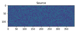
Not much to look at!

Saving and loading a model

Now let’s save this model and load it back up.

with tempfile.NamedTemporaryFile(suffix='.pth', delete=True) as f:
    loc = model.save(f.name)
    reloaded_dict = torch.load(f.name)

    print(reloaded_dict.keys())

    new_model = nussl.ml.SeparationModel(reloaded_dict['config'])
    new_model.load_state_dict(reloaded_dict['state_dict'])

    print(new_model)

dict_keys(['state_dict', 'config', 'nussl_version'])
SeparationModel(
  (layers): ModuleDict(
    (my_estimates): Mask()
    (my_log_spec): AmplitudeToDB()
    (my_mask): Embedding(
      (linear): Linear(in_features=129, out_features=387, bias=True)
    )
    (my_norm): BatchNorm(
      (batch_norm): BatchNorm1d(1, eps=1e-05, momentum=0.1, affine=True, track_running_stats=True)
    )
  )
)
Number of parameters: 50312

When models are saved, both the config AND the weights are saved. Both of these can be easily loaded back into a new SeparationModel object.

Custom modules

There’s also straightforward support for custom modules that don’t exist in nussl but rather exist in the end-user code. These can be registered with SeparationModel easily. Let’s build a custom module and register it with a copy of our existing model. Let’s make this module a lambda, which takes in some arbitrary function and runs it on the input. We’ll call it LambdaLayer:

class LambdaLayer(torch.nn.Module):
    def __init__(self, func):
        self.func = func
        super().__init__()

    def forward(self, data):
        return self.func(data)


def print_shape(x):
    print(f'Shape is {x.shape}')


lamb = LambdaLayer(print_shape)
output = lamb(mix_magnitude)

Shape is torch.Size([1, 400, 129, 1])

Now let’s put it into a copy of our model and update the connections so that it prints for every layer.

# Copy our previous modules and add our new Lambda class
new_modules = copy.deepcopy(modules)
new_modules['lambda'] = {
    'class': 'LambdaLayer',
    'args': {
        'func': print_shape
    }
}

new_connections = [
    ['my_log_spec', ['mix_magnitude', ]],
    ['lambda', ['mix_magnitude', ]],
    ['lambda', ['my_log_spec', ]],
    ['my_norm', ['my_log_spec', ]],
    ['lambda', ['my_norm', ]],
    ['my_mask', ['my_norm', ]],
    ['lambda', ['my_mask', ]],
    ['my_estimates', ['my_mask', 'mix_magnitude']],
    ['lambda', ['my_estimates', ]]
]

new_config = {
    'modules': new_modules,
    'connections': new_connections,
    'output': ['my_estimates', 'my_mask']
}

But right now, SeparationModel doesn’t know about our LambdaLayer class! So, let’s make it aware by registering the module with nussl:

nussl.ml.register_module(LambdaLayer)
print_existing_modules()

nussl.ml.modules contents:
--------------------------
AmplitudeToDB
BatchNorm
Concatenate
ConvolutionalStack2D
DualPath
DualPathBlock
Embedding
Expand
FilterBank
GaussianMixtureTorch
InstanceNorm
LambdaLayer
LayerNorm
LearnedFilterBank
Mask
MelProjection
RecurrentStack
STFT
ShiftAndScale
Split
blocks
filter_bank

Now LambdaLayer is a registered module! Let’s build the SeparationModel and put some data through it:

verbose_model = nussl.ml.SeparationModel(new_config)
output = verbose_model(data)

Shape is torch.Size([1, 400, 129, 1])
Shape is torch.Size([1, 400, 129, 1])
Shape is torch.Size([1, 400, 129, 1])
Shape is torch.Size([1, 400, 129, 1, 3])
Shape is torch.Size([1, 400, 129, 1, 3])

We can see the outputs of the Lambda layer recurring after each connection. (Note: that because we used a non-serializable argument (the function, func) to the LambdaLayer, this model won’t save without special handling!)

Alright, now let’s see how to use some actual audio data with our model…

Handling data

As described in the datasets tutorial, the heart of nussl data handling is BaseDataset and its associated subclasses. We built a simple one in that tutorial that just produced random sine waves. Let’s grab it again:

def make_sine_wave(freq, sample_rate, duration):
    dt = 1 / sample_rate
    x = np.arange(0.0, duration, dt)
    x = np.sin(2 * np.pi * freq * x)
    return x


class SineWaves(nussl.datasets.BaseDataset):
    def __init__(self, *args, num_sources=3, num_frequencies=20, **kwargs):
        self.num_sources = num_sources
        self.frequencies = np.random.choice(
            np.arange(110, 4000, 100), num_frequencies,
            replace=False)

        super().__init__(*args, **kwargs)

    def get_items(self, folder):
        # ignore folder and return a list
        # 100 items in this dataset
        items = list(range(100))
        return items

    def process_item(self, item):
        # we're ignoring ``items`` and making
        # sums of random sine waves
        sources = {}
        freqs = np.random.choice(
            self.frequencies, self.num_sources,
            replace=False)
        for i in range(self.num_sources):
            freq = freqs[i]
            _data = make_sine_wave(freq, self.sample_rate, 2)
            # this is a helper function in BaseDataset for
            # making an audio signal from data
            signal = self._load_audio_from_array(_data)
            signal.path_to_input_file = f'{item}.wav'
            sources[f'sine{i}'] = signal * 1 / self.num_sources

        mix = sum(sources.values())

        metadata = {
            'frequencies': freqs
        }

        output = {
            'mix': mix,
            'sources': sources,
            'metadata': metadata
        }
        return output

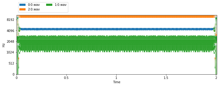
As a reminder, this dataset makes random mixtures of sine waves with fundamental frequencies between 110 Hz and 4000 Hz. Let’s now set it up with appropriate STFT parameters that result in 129 frequencies in the spectrogram.

nussl.utils.seed(0)  # make sure this does the same thing each time

# We're not reading data, so we can 'ignore' the folder
folder = 'ignored'

stft_params = nussl.STFTParams(window_length=256, hop_length=64)

sine_wave_dataset = SineWaves(
    folder, sample_rate=8000, stft_params=stft_params
)

item = sine_wave_dataset[0]


def visualize_and_embed(sources, y_axis='mel'):
    plt.figure(figsize=(10, 4))
    plt.subplot(111)
    nussl.utils.visualize_sources_as_masks(
        sources, db_cutoff=-60, y_axis=y_axis)
    plt.tight_layout()
    plt.show()

    nussl.play_utils.multitrack(sources, ext='.wav')


visualize_and_embed(item['sources'])
print(item['metadata'])

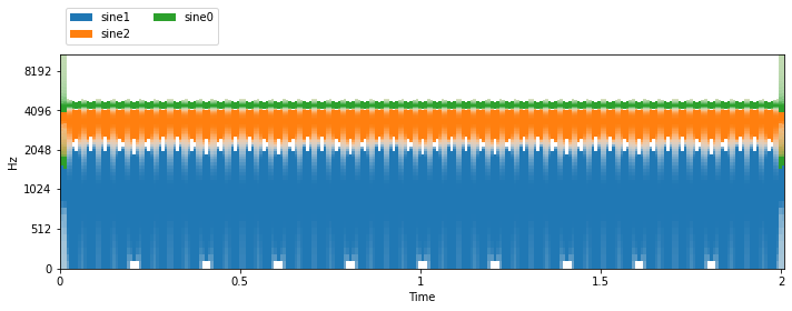
{'frequencies': array([1610,  310, 1210])}

Let’s check the shape of the mix stft:

item['mix'].stft().shape

(129, 251, 1)

Great! There’s 129 frequencies and 251 frames and 1 audio channel. To put it into our model though, we need the STFT in the right shape, and we also need some training data. Let’s use some of nussl’s transforms to do this. Specifically, we’ll use the PhaseSensitiveSpectrumApproximation and the ToSeparationModel transforms. We’ll also use the MagnitudeWeights transform in case we want to use deep clustering loss functions.

folder = 'ignored'
stft_params = nussl.STFTParams(window_length=256, hop_length=64)
tfm = nussl.datasets.transforms.Compose([
    nussl.datasets.transforms.PhaseSensitiveSpectrumApproximation(),
    nussl.datasets.transforms.MagnitudeWeights(),
    nussl.datasets.transforms.ToSeparationModel()
])

sine_wave_dataset = SineWaves(
    folder, sample_rate=8000, stft_params=stft_params,
    transform=tfm
)

# Let's inspect the 0th item from the dataset
item = sine_wave_dataset[0]
item.keys()

dict_keys(['index', 'mix_magnitude', 'ideal_binary_mask', 'source_magnitudes', 'weights'])

Now the item has all the keys that SeparationModel needs. The ToSeparationModel transform set everything up for us: it set up the dictionary from SineWaves.process_item() exactly as we needed it. It swapped the frequency and sequence length dimension appropriately, and made them all torch Tensors:

item['mix_magnitude'].shape

torch.Size([251, 129, 1])

We still need to add a batch dimension and make everything have float type though. So let’s do that for each key, if the key is a torch Tensor:

for key in item:
    if torch.is_tensor(item[key]):
        item[key] = item[key].unsqueeze(0).float()

item['mix_magnitude'].shape

torch.Size([1, 251, 129, 1])

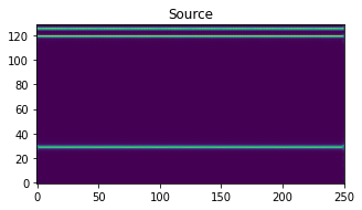
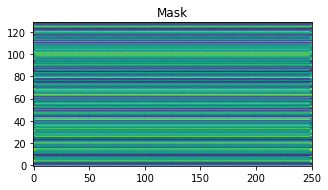
Now we can pass this through our model:

output = model(item)

i = 0
plt.figure(figsize=(5, 5))
plt.imshow(
    output['my_estimates'][0, ..., 0, i].T.cpu().data.numpy(),
    origin='lower')
plt.title("Source")
plt.show()

plt.figure(figsize=(5, 5))
plt.imshow(
    output['my_mask'][0, ..., 0, i].T.cpu().data.numpy(),
    origin='lower')
plt.title("Mask")
plt.show()

We’ve now seen how to use nussl transforms, datasets, and SeparationModel together to make a forward pass. But so far our model does nothing practical; let’s see how to train the model so it actually does something.

Closures and loss functions

nussl trains models via closures, which define the forward and backward passes for a model on a single batch. Closures use loss functions within them, which compute the loss on a single batch. There are a bunch of common loss functions already in nussl.

def print_existing_losses():
    excluded = ['nn', 'torch', 'combinations', 'permutations']
    print('nussl.ml.train.loss contents:')
    print('-----------------------------')
    existing_losses = [x for x in dir(nussl.ml.train.loss) if
                       x not in excluded and not x.startswith('__')]
    print('\n'.join(existing_losses))


print_existing_losses()

nussl.ml.train.loss contents:
-----------------------------
CombinationInvariantLoss
DeepClusteringLoss
KLDivLoss
L1Loss
MSELoss
PermutationInvariantLoss
SISDRLoss
WhitenedKMeansLoss

In addition to standard loss functions for spectrograms, like L1 Loss and MSE, there is also an SDR loss for time series audio, as well as permutation invariant versions of these losses for training things like speaker separation networks. See the API docs for more details on all of these loss functions. A closure uses these loss functions in a simple way. For example, here is the code for training a model with a closure:

from nussl.ml.train.closures import Closure
from nussl.ml.train import BackwardsEvents


class TrainClosure(Closure):
    """
    This closure takes an optimization step on a SeparationModel object given a
    loss.

    Args:
        loss_dictionary (dict): Dictionary containing loss functions and specification.
        optimizer (torch Optimizer): Optimizer to use to train the model.
        model (SeparationModel): The model to be trained.
    """

    def __init__(self, loss_dictionary, optimizer, model):
        super().__init__(loss_dictionary)
        self.optimizer = optimizer
        self.model = model

    def __call__(self, engine, data):
        self.model.train()
        self.optimizer.zero_grad()

        output = self.model(data)

        loss_ = self.compute_loss(output, data)
        loss_['loss'].backward()
        engine.fire_event(BackwardsEvents.BACKWARDS_COMPLETED)
        self.optimizer.step()
        loss_ = {key: loss_[key].item() for key in loss_}

        return loss_

So, this closure takes some data and puts it through the model, then calls self.compute_loss on the result, fires an event on the ignite engine, and then steps the optimizer on the loss. This is a standard PyTorch training loop. The magic here is happening in self.compute_loss, which comes from the parent class Closure.

Loss dictionary

The parent class Closure takes a loss dictionary which defines the losses that get computed on the output of the model. The loss dictionary has the following format:

loss_dictionary = {
        'LossClassName': {
            'weight': [how much to weight the loss in the sum, defaults to 1],
            'keys': [key mapping items in dictionary to arguments to loss],
            'args': [any positional arguments to the loss class],
            'kwargs': [keyword arguments to the loss class],
        }
    }

For example, one possible loss could be:

loss_dictionary = {
    'DeepClusteringLoss': {
        'weight': .2,
    },
    'PermutationInvariantLoss': {
        'weight': .8,
        'args': ['L1Loss']
    }
}

This will apply the deep clustering and a permutation invariant L1 loss to the output of the model. So, how does the model know what to compare? Each loss function is a class in nussl, and each class has an attribute called DEFAULT_KEYS, This attribute tells the Closure how to use the forward pass of the loss function. For example, this is the code for the L1 Loss:

from torch import nn


class L1Loss(nn.L1Loss):
    DEFAULT_KEYS = {'estimates': 'input', 'source_magnitudes': 'target'}

L1Loss is defined in PyTorch and has the following example for its forward pass:

>>> loss = nn.L1Loss()
>>> input = torch.randn(3, 5, requires_grad=True)
>>> target = torch.randn(3, 5)
>>> output = loss(input, target)
>>> output.backward()

The arguments to the function are input and target. So the mapping from the dictionary provided by our dataset and model jointly is to use my_estimates (like we defined above) as the input and source_magnitudes (what we are trying to match) as the target. This results in the DEFAULT_KEYS you see above. Alternatively, you can pass the mapping between the dictionary and the arguments to the loss function directly into the loss dictionary like so:

loss_dictionary = {
    'L1Loss': {
        'weight': 1.0,
        'keys': {
            'my_estimates': 'input',
            'source_magnitudes': 'target',
        }
    }
}

Great, now let’s use this loss dictionary in a Closure and see what happens.

closure = nussl.ml.train.closures.Closure(loss_dictionary)
closure.losses

[(L1Loss(),
  1.0,
  {'my_estimates': 'input', 'source_magnitudes': 'target'},
  'L1Loss')]

The closure was instantiated with the losses. Calling closure.compute_loss results in the following:

output = model(item)
loss_output = closure.compute_loss(output, item)
for key, val in loss_output.items():
    print(key, val)

L1Loss tensor(0.0037, grad_fn=<L1LossBackward>)
loss tensor(0.0037, grad_fn=<AddBackward0>)

The output is a dictionary with the loss item corresponding to the total (summed) loss and the other keys corresponding to the individual losses.

Custom loss functions

Loss functions can be registered with the Closure in the same way that modules are registered with SeparationModel:

class MeanDifference(torch.nn.Module):
    DEFAULT_KEYS = {'my_estimates': 'input', 'source_magnitudes': 'target'}

    def __init__(self):
        super().__init__()

    def forward(self, input, target):
        return torch.abs(input.mean() - target.mean())


nussl.ml.register_loss(MeanDifference)
print_existing_losses()

nussl.ml.train.loss contents:
-----------------------------
CombinationInvariantLoss
DeepClusteringLoss
KLDivLoss
L1Loss
MSELoss
MeanDifference
PermutationInvariantLoss
SISDRLoss
WhitenedKMeansLoss

Now this loss can be used in a closure:

new_loss_dictionary = {
    'MeanDifference': {}
}

new_closure = nussl.ml.train.closures.Closure(new_loss_dictionary)
new_closure.losses

output = model(item)
loss_output = new_closure.compute_loss(output, item)
for key, val in loss_output.items():
    print(key, val)

MeanDifference tensor(0.0012, grad_fn=<AbsBackward>)
loss tensor(0.0012, grad_fn=<AddBackward0>)

Optimizing the model

We now have a loss. We can then put it backwards through the model and take a step forward on the model with an optimizer. Let’s define an optimizer (we’ll use Adam), and then use it to take a step on the model:

optimizer = torch.optim.Adam(model.parameters(), lr=.001)

optimizer.zero_grad()
output = model(item)
loss_output = closure.compute_loss(output, item)
loss_output['loss'].backward()
optimizer.step()
print(loss_output)

{'L1Loss': tensor(0.0037, grad_fn=<L1LossBackward>), 'loss': tensor(0.0037, grad_fn=<AddBackward0>)}

Cool, we did a single step. Instead of manually defining this all above, we can instead use the TrainClosure from nussl.

train_closure = nussl.ml.train.closures.TrainClosure(
    loss_dictionary, optimizer, model
)

The __call__ function of the closure takes an engine as well as the batch data. Since we don’t currently have an engine object (more on that below), let’s just pass None. We can run this on a batch:

train_closure(None, item)

{'L1Loss': 0.003581754630431533, 'loss': 0.003581754630431533}

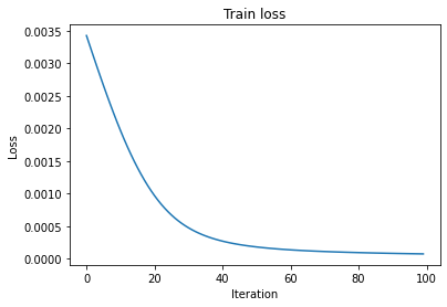
We can run this a bunch of times and watch the loss go down.

loss_history = []
n_iter = 100

for i in range(n_iter):
    loss_output = train_closure(None, item)
    loss_history.append(loss_output['loss'])

plt.plot(loss_history)
plt.title('Train loss')
plt.xlabel('Iteration')
plt.ylabel('Loss')
plt.show()

Note that there is also a ValidationClosure which does not take an optimization step but only computes the loss.

Let’s look at the model output now!

output = model(item)

for i in range(output['my_estimates'].shape[-1]):
    plt.figure(figsize=(10, 5))
    plt.subplot(121)
    plt.imshow(
        output['my_estimates'][0, ..., 0, i].T.cpu().data.numpy(),
        origin='lower')
    plt.title("Source")

    plt.subplot(122)
    plt.imshow(
        output['my_mask'][0, ..., 0, i].T.cpu().data.numpy(),
        origin='lower')
    plt.title("Mask")
    plt.show()

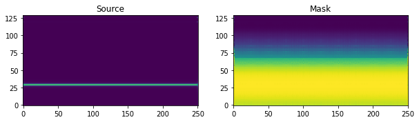
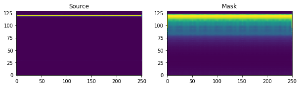
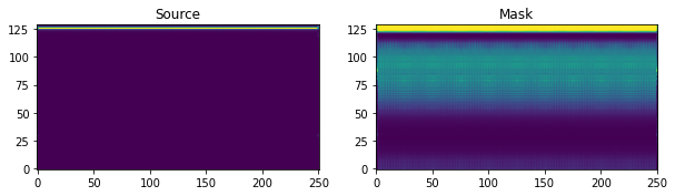
Hey! That looks a lot better! We’ve now overfit the model to a single item in the dataset. Now, let’s do it at scale by using a PyTorch Ignite engines with the functionality in nussl.ml.train.

Ignite Engines

nussl uses PyTorch Ignite to power its training functionality. PyTorch At the heart of Ingite is the Engine object. An Engine contains a lot of functionality for iterating through a dataset and feeding data to a model. What makes Ignite so desireable is that we can define all of the things we need to train a model ahead of time, the the Ignite engine will run the code to train the model for us. This saves us a lot of time writing boilerplate code for training. nussl also provides a lot of boilerplate code for training source separation models, specifically.

To use Ignite with nussl, the only thing we need to to define is a closure. A closure defines a pass through the model for a single batch. The rest of the details, such as queueing up data, are taken care of by torch.utils.data.DataLoader and the engine object. All of the state regarding a training run, such as the epoch number, the loss history, etc, is kept in the engine’s state at engine.state.

nussl provides a helper function to build a standard engine with a lot of nice functionality like keeping track of loss history, preparing the batches properly, setting up the train and validation closures. This function is create_train_and_validation_engines().

It’s also possible to add attach handlers to an Engine for further functionality. These handlers make use of the engine’s state. nussl comes with several of these:

1. add_validate_and_checkpoint: Adds a pass on the validation data and checkpoints the model based on the validation loss to either best (if this was the lowest validation loss model) or latest.

2. add_stdout_handler: Prints some handy information after each epoch.

3. add_tensorboard_handler: Logs loss data to tensorboard.

See the API documentation for further details on these handlers.

Putting it all together

Let’s put this all together. Let’s build the dataset, model and optimizer, train and validation closures, and engines. Let’s also use the GPU if it’s available.

# define everything as before
modules = {
    'mix_magnitude': {},
    'log_spec': {
        'class': 'AmplitudeToDB'
    },
    'norm': {
        'class': 'BatchNorm',
    },
    'mask': {
        'class': 'Embedding',
        'args': {
            'num_features': num_features,
            'hidden_size': num_features,
            'embedding_size': num_sources,
            'activation': mask_activation,
            'num_audio_channels': num_audio_channels,
            'dim_to_embed': [2, 3]  # embed the frequency dimension (2) for all audio channels (3)
        }
    },
    'estimates': {
        'class': 'Mask',
    },
}

connections = [
    ['log_spec',    ['mix_magnitude',       ]],
    ['norm',        ['log_spec',            ]],
    ['mask',        ['norm',                ]],
    ['estimates',   ['mask', 'mix_magnitude']]
]

# define the outputs
output = ['estimates', 'mask']

config = {
    'modules': modules,
    'connections': connections,
    'output': output
}

BATCH_SIZE = 5
LEARNING_RATE = 1e-3
OUTPUT_FOLDER = os.path.expanduser('~/.nussl/tutorial/sinewave')
RESULTS_DIR = os.path.join(OUTPUT_FOLDER, 'results')
NUM_WORKERS = 2
DEVICE = 'cuda' if torch.cuda.is_available() else 'cpu'

shutil.rmtree(os.path.join(RESULTS_DIR), ignore_errors=True)

os.makedirs(RESULTS_DIR, exist_ok=True)
os.makedirs(OUTPUT_FOLDER, exist_ok=True)

# adjust logging so we see output of the handlers
logger = logging.getLogger()
logger.setLevel(logging.INFO)

# Put together data
stft_params = nussl.STFTParams(window_length=256, hop_length=64)
tfm = nussl.datasets.transforms.Compose([
    nussl.datasets.transforms.PhaseSensitiveSpectrumApproximation(),
    nussl.datasets.transforms.MagnitudeWeights(),
    nussl.datasets.transforms.ToSeparationModel()
])
sine_wave_dataset = SineWaves(
    'ignored', sample_rate=8000, stft_params=stft_params,
    transform=tfm
)
dataloader = torch.utils.data.DataLoader(
    sine_wave_dataset, batch_size=BATCH_SIZE
)

# Build our simple model
model = nussl.ml.SeparationModel(config).to(DEVICE)

# Build an optimizer
optimizer = torch.optim.Adam(model.parameters(), lr=LEARNING_RATE)

# Set up loss functions and closure
# We'll use permutation invariant loss since we don't
# care what order the sine waves get output in, just that
# they are different.
loss_dictionary = {
    'PermutationInvariantLoss': {
        'weight': 1.0,
        'args': ['L1Loss']
    }
}

train_closure = nussl.ml.train.closures.TrainClosure(
    loss_dictionary, optimizer, model
)
val_closure = nussl.ml.train.closures.ValidationClosure(
    loss_dictionary, model
)

# Build the engine and add handlers
train_engine, val_engine = nussl.ml.train.create_train_and_validation_engines(
    train_closure, val_closure, device=DEVICE
)
nussl.ml.train.add_validate_and_checkpoint(
    OUTPUT_FOLDER, model, optimizer, sine_wave_dataset, train_engine,
    val_data=dataloader, validator=val_engine
)
nussl.ml.train.add_stdout_handler(train_engine, val_engine)

Cool! We built an engine! (Note the distinction between using the original dataset object and using the dataloader object.)

Now to train it, all we have to do is run the engine. Since our SineWaves dataset makes mixes “on the fly” (i.e., every time we get an item, the dataset will return a mix of random sine waves), it is impossible to loop through the whole dataset, and therefore there is no concept of an epoch. In this case, we will instead define an arbitrary epoch_length of 1000 and pass that value to train_engine. After one epoch, the validation will be run and everything will get printed by the stdout handler.

Let’s see it run:

train_engine.run(dataloader, epoch_length=1000)

INFO:root:

EPOCH SUMMARY
~~~~~~~~~~~~~~~~~~~~~~~~~~~~~~
- Epoch number: 0001 / 0001
- Training loss:   0.001197
- Validation loss: 0.000683
- Epoch took: 00:02:11
- Time since start: 00:02:11
~~~~~~~~~~~~~~~~~~~~~~~~~~~~~~
Saving to /home/pseetharaman/.nussl/tutorial/sinewave/checkpoints/best.model.pth.
Output @ /home/pseetharaman/.nussl/tutorial/sinewave

INFO:ignite.engine.engine.Engine:Engine run complete. Time taken 00:02:11

State:
        iteration: 1000
        epoch: 1
        epoch_length: 1000
        max_epochs: 1
        output: <class 'dict'>
        batch: <class 'dict'>
        metrics: <class 'dict'>
        dataloader: <class 'torch.utils.data.dataloader.DataLoader'>
        seed: 12
        epoch_history: <class 'dict'>
        iter_history: <class 'dict'>
        past_iter_history: <class 'dict'>
        saved_model_path: /home/pseetharaman/.nussl/tutorial/sinewave/checkpoints/best.model.pth
        output_folder: /home/pseetharaman/.nussl/tutorial/sinewave

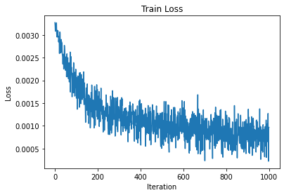
We can check out the loss over each iteration in the single epoch by examining the state:

plt.plot(train_engine.state.iter_history['loss'])
plt.xlabel('Iteration')
plt.ylabel('Loss')
plt.title('Train Loss')
plt.show()

Let’s also see what got saved in the output folder:

!tree {OUTPUT_FOLDER}

/home/pseetharaman/.nussl/tutorial/sinewave
├── checkpoints
│   ├── best.model.pth
│   ├── best.optimizer.pth
│   ├── latest.model.pth
│   └── latest.optimizer.pth
└── results

2 directories, 4 files

So the models and optimizers got saved! Let’s load back one of these models and see what’s in it.

What’s in a model?

After we’re finished training the model, it will be saved by our add_validate_and_checkpoint handler. What gets saved in our model? Let’s see:

saved_model = torch.load(train_engine.state.saved_model_path)
print(saved_model.keys())

dict_keys(['state_dict', 'config', 'metadata', 'nussl_version'])

As expected, there’s the state_dict containing the weights of the trained model, the config containing the configuration of the model. There also a metadata key in the saved model. Let’s check out the metadata…

print(saved_model['metadata'].keys())

dict_keys(['stft_params', 'sample_rate', 'num_channels', 'folder', 'transforms', 'trainer.state_dict', 'trainer.state.epoch_history'])

There’s a whole bunch of stuff related to training, like the folder it was trained on, the state dictionary of the engine used to train the model, the loss history for each epoch (not each iteration - that’s too big).

There are also keys that are related to the parameters of the AudioSignal. Namely, stft_params, sample_rate, and num_channels. These are used by nussl to prepare an AudioSignal object to be put into a deep learning based separation algorithm. There’s also a transforms key - this is used by nussl to construct the input dictionary at inference time on an AudioSignal so that the data going into the model matches how it was given during training time. Let’s look at each of these:

for key in saved_model['metadata']:
    print(f"{key}: {saved_model['metadata'][key]}")

stft_params: STFTParams(window_length=256, hop_length=64, window_type=None)
sample_rate: 8000
num_channels: 1
folder: ignored
transforms: Compose(
    PhaseSensitiveSpectrumApproximation(mix_key = mix, source_key = sources)
    <nussl.datasets.transforms.MagnitudeWeights object at 0x7fe70c100ed0>
    ToSeparationModel()
)
trainer.state_dict: {'epoch': 1, 'epoch_length': 1000, 'max_epochs': 1, 'output': {'PermutationInvariantLoss': 0.000967394735198468, 'loss': 0.000967394735198468}, 'metrics': {}, 'seed': 12}
trainer.state.epoch_history: {'validation/PermutationInvariantLoss': [0.000682936332304962], 'validation/loss': [0.000682936332304962], 'train/PermutationInvariantLoss': [0.0011968749410734745], 'train/loss': [0.0011968749410734745]}

Importantly, everything saved with the model makes training it entirely reproduceable. We have everything we need to recreate another model exactly like this if we need to.

Now that we’ve trained our toy model, let’s move on to actually using and evaluating it.

Using and evaluating a trained model

In this tutorial, we built very simple a deep mask estimation network. There is a corresponding separation algorithm in nussl for using deep mask estimation networks. Let’s build our dataset again, this time without transforms, so we have access to the actual AudioSignal objects. Then let’s instantiate the separation algorithm and use it to separate an item from the dataset.

tt_dataset = SineWaves(
    'ignored', sample_rate=8000
)
tt_dataset.frequencies = sine_wave_dataset.frequencies

item = tt_dataset[0]  # <-- This is an AugioSignal obj

MODEL_PATH = os.path.join(OUTPUT_FOLDER, 'checkpoints/best.model.pth')

separator = nussl.separation.deep.DeepMaskEstimation(
    item['mix'], model_path=MODEL_PATH
)
estimates = separator()

visualize_and_embed(estimates)

Evaluation in parallel

We’ll usually want to run many mixtures through the model, separate, and get evaluation metrics like SDR, SIR, and SAR. We can do that with the following bit of code:

# make a separator with an empty audio signal initially
# this one will live on gpu (if one exists) and be used in a
# threadpool for speed
dme = nussl.separation.deep.DeepMaskEstimation(
    nussl.AudioSignal(), model_path=MODEL_PATH, device='cuda'
)


def forward_on_gpu(audio_signal):
    # set the audio signal of the object to this item's mix
    dme.audio_signal = audio_signal
    masks = dme.forward()
    return masks


def separate_and_evaluate(item, masks):
    separator = nussl.separation.deep.DeepMaskEstimation(item['mix'])
    estimates = separator(masks)

    evaluator = nussl.evaluation.BSSEvalScale(
        list(item['sources'].values()), estimates,
        compute_permutation=True,
        source_labels=['sine1', 'sine2', 'sine3']
    )
    scores = evaluator.evaluate()
    output_path = os.path.join(
        RESULTS_DIR, f"{item['mix'].file_name}.json"
    )
    with open(output_path, 'w') as f:
        json.dump(scores, f)

pool = ThreadPoolExecutor(max_workers=NUM_WORKERS)
for i, item in enumerate(tqdm.tqdm(tt_dataset)):
    masks = forward_on_gpu(item['mix'])
    if i == 0:
        separate_and_evaluate(item, masks)
    else:
        pool.submit(separate_and_evaluate, item, masks)
pool.shutdown(wait=True)

json_files = glob.glob(f"{RESULTS_DIR}/*.json")
df = nussl.evaluation.aggregate_score_files(json_files)
report_card = nussl.evaluation.report_card(
    df, notes="Testing on sine waves", report_each_source=True)
print(report_card)

/home/pseetharaman/Dropbox/research/nussl_refactor/nussl/separation/base/separation_base.py:71: UserWarning: input_audio_signal has no data!
  warnings.warn('input_audio_signal has no data!')
/home/pseetharaman/Dropbox/research/nussl_refactor/nussl/core/audio_signal.py:445: UserWarning: Initializing STFT with data that is non-complex. This might lead to weird results!
  warnings.warn('Initializing STFT with data that is non-complex. '
 96%|█████████▌| 96/100 [00:04<00:00, 17.45it/s]/home/pseetharaman/Dropbox/research/nussl_refactor/nussl/evaluation/bss_eval.py:33: RuntimeWarning: divide by zero encountered in log10
  srr = -10 * np.log10((1 - (1/alpha)) ** 2)
100%|██████████| 100/100 [00:05<00:00, 19.65it/s]

                                MEAN +/- STD OF METRICS

┌─────────┬──────────────────┬──────────────────┬──────────────────┬──────────────────┐
│ METRIC  │     OVERALL      │      SINE1       │      SINE2       │      SINE3       │
╞═════════╪══════════════════╪══════════════════╪══════════════════╪══════════════════╡
│ #       │       300        │       100        │       100        │       100        │
├─────────┼──────────────────┼──────────────────┼──────────────────┼──────────────────┤
│ SI-SDR  │  14.83 +/- 15.89 │  15.44 +/- 14.83 │  14.20 +/- 17.41 │  14.85 +/- 15.44 │
├─────────┼──────────────────┼──────────────────┼──────────────────┼──────────────────┤
│ SI-SIR  │  25.39 +/- 19.97 │  25.79 +/- 18.48 │  24.89 +/- 21.90 │  25.50 +/- 19.57 │
├─────────┼──────────────────┼──────────────────┼──────────────────┼──────────────────┤
│ SI-SAR  │  19.46 +/- 14.75 │  19.27 +/- 14.17 │  19.26 +/- 15.35 │  19.84 +/- 14.86 │
├─────────┼──────────────────┼──────────────────┼──────────────────┼──────────────────┤
│ SD-SDR  │   8.68 +/- 21.89 │   8.65 +/- 21.83 │   8.38 +/- 22.88 │   9.02 +/- 21.15 │
├─────────┼──────────────────┼──────────────────┼──────────────────┼──────────────────┤
│ SNR     │  15.13 +/- 10.91 │  15.23 +/- 10.46 │  15.23 +/- 11.41 │  14.92 +/- 10.96 │
├─────────┼──────────────────┼──────────────────┼──────────────────┼──────────────────┤
│ SRR     │  20.46 +/- 29.52 │  20.31 +/- 29.74 │  20.62 +/- 30.97 │  20.45 +/- 28.06 │
├─────────┼──────────────────┼──────────────────┼──────────────────┼──────────────────┤
│ SI-SDRi │  17.84 +/- 15.89 │  18.45 +/- 14.83 │  17.21 +/- 17.41 │  17.86 +/- 15.44 │
├─────────┼──────────────────┼──────────────────┼──────────────────┼──────────────────┤
│ SD-SDRi │  11.69 +/- 21.89 │  11.66 +/- 21.83 │  11.39 +/- 22.88 │  12.03 +/- 21.15 │
├─────────┼──────────────────┼──────────────────┼──────────────────┼──────────────────┤
│ SNRi    │  18.14 +/- 10.91 │  18.24 +/- 10.46 │  18.24 +/- 11.41 │  17.93 +/- 10.96 │
└─────────┴──────────────────┴──────────────────┴──────────────────┴──────────────────┘

                                   MEDIAN OF METRICS

┌─────────┬──────────────────┬──────────────────┬──────────────────┬──────────────────┐
│ METRIC  │     OVERALL      │      SINE1       │      SINE2       │      SINE3       │
╞═════════╪══════════════════╪══════════════════╪══════════════════╪══════════════════╡
│ #       │       300        │       100        │       100        │       100        │
├─────────┼──────────────────┼──────────────────┼──────────────────┼──────────────────┤
│ SI-SDR  │       19.40      │       19.73      │       19.16      │       19.16      │
├─────────┼──────────────────┼──────────────────┼──────────────────┼──────────────────┤
│ SI-SIR  │       28.23      │       28.29      │       28.53      │       27.48      │
├─────────┼──────────────────┼──────────────────┼──────────────────┼──────────────────┤
│ SI-SAR  │       22.07      │       21.56      │       22.41      │       22.11      │
├─────────┼──────────────────┼──────────────────┼──────────────────┼──────────────────┤
│ SD-SDR  │       16.27      │       17.13      │       16.12      │       15.66      │
├─────────┼──────────────────┼──────────────────┼──────────────────┼──────────────────┤
│ SNR     │       16.87      │       17.68      │       16.57      │       16.05      │
├─────────┼──────────────────┼──────────────────┼──────────────────┼──────────────────┤
│ SRR     │       26.03      │       26.08      │       26.32      │       24.06      │
├─────────┼──────────────────┼──────────────────┼──────────────────┼──────────────────┤
│ SI-SDRi │       22.42      │       22.74      │       22.17      │       22.17      │
├─────────┼──────────────────┼──────────────────┼──────────────────┼──────────────────┤
│ SD-SDRi │       19.28      │       20.14      │       19.13      │       18.67      │
├─────────┼──────────────────┼──────────────────┼──────────────────┼──────────────────┤
│ SNRi    │       19.88      │       20.70      │       19.59      │       19.06      │
└─────────┴──────────────────┴──────────────────┴──────────────────┴──────────────────┘

                                         NOTES

Testing on sine waves

We parallelized the evaluation across 2 workers, kept two copies of the separator, one of which lives on the GPU, and the other which lives on the CPU. The GPU one does a forward pass in its own thread and then hands it to the other separator which actually computes the estimates and evaluates the metrics in parallel. After we’re done, we aggregate all the results (each of which was saved to a JSON file) using nussl.evaluation.aggregate_score_files and then use the nussl report card at nussl.evaluation.report_card to view the results. We also now have the results as a pandas DataFrame:

df

	source	file	SI-SDR	SI-SIR	SI-SAR	SD-SDR	SNR	SRR	SI-SDRi	SD-SDRi	SNRi
0	sine3	46.wav.json	-20.328155	-8.004939	-20.066033	-40.275110	0.039984	-40.230923	-17.317855	-37.264810	3.050284
1	sine3	95.wav.json	28.667780	47.823142	28.720856	25.991488	26.282122	29.363641	31.678080	29.001788	29.292422
2	sine3	10.wav.json	33.812458	51.036624	33.895541	33.172820	33.243078	41.807216	36.822758	36.183120	36.253378
3	sine3	83.wav.json	9.767297	9.882167	25.600388	9.746169	9.940989	32.886040	12.777597	12.756469	12.951289
4	sine3	22.wav.json	6.323363	23.420462	6.408937	-19.179230	0.894722	-19.166980	9.333663	-16.168930	3.905022
...	...	...	...	...	...	...	...	...	...	...	...
295	sine1	0.wav.json	20.901103	36.092488	21.034547	20.883094	20.933421	44.715190	23.911403	23.893394	23.943721
296	sine1	63.wav.json	18.457849	34.462413	18.568215	17.429336	17.949669	24.189192	21.468149	20.439636	20.959969
297	sine1	92.wav.json	2.070333	2.341293	14.253886	-7.646593	2.669284	-7.156396	5.080632	-4.636293	5.679584
298	sine1	37.wav.json	-16.620665	12.170543	-16.614925	-49.367983	0.027190	-49.365675	-13.610365	-46.357683	3.037490
299	sine1	43.wav.json	19.687632	20.537881	27.188207	19.680721	19.716579	47.666603	22.697932	22.691021	22.726879

300 rows × 11 columns

Finally, we can look at the structure of the output folder again, seeing there are now 100 entries under results corresponding to each item in sine_wave_dataset:

!tree --filelimit 20 {OUTPUT_FOLDER}

/home/pseetharaman/.nussl/tutorial/sinewave
├── checkpoints
│   ├── best.model.pth
│   ├── best.optimizer.pth
│   ├── latest.model.pth
│   └── latest.optimizer.pth
└── results [100 entries exceeds filelimit, not opening dir]

2 directories, 4 files

end_time = time.time()
time_taken = end_time - start_time
print(f'Time taken: {time_taken:.4f} seconds')

Time taken: 169.6379 seconds